Dec 8, 2016

Finding differences between bacterial strains 100 bases at a time.

This work was conducted mostly by my research assistant Yuhan Hao.

We have recently been using Bowtie2 for sequence comparisons related to shotgun metagenomics, where we directly sequence samples that contain mixtures of DNA from different organisms, with no PCR. Bowtie2 alignments can be made very stringently (>90% identity), and computed very rapidly for large data files with hundreds of millions of sequence reads. This allows us to identify DNA fragments by species and by gene function, provided we have a well-annotated database that contains DNA sequences from similar microbes. I know that MetaPhlan and other tools already do this, but I want to focus on the difference between bacteria (and viruses) at the strain level.

I have been playing around with the idea of constructing a database that will give strain-specific identification for human-associated microbes using Bowtie2 alignments with shotgun metagenomic data. There are plenty of sources for bacterial genome sequences, but the PATRIC database has a very good collection of human pathogen genomes. However the database is very redundant - with dozens or even hundreds of different strains for the same species, and the whole thing is too large to build into a Bowtie database (>350 Gb). So I am looking at ways to eliminate redundancy from the database while retaining high sensitivity at the species level to identify any sequence fragment, not just specific marker genes,  and the ability to make strain-specific alignments. So I want to identify which genome fragments have shared sequences among a group of strains within a single species and which fragments are unique to each strain.

Since our sequence reads are usually ~100 bases, We are looking the similarity between bacterial strains when the genome is chopped into 100 bp pieces.

Bowtie2 can be limited to only perfect alignments (100 bases with zero mismatches) using the parameters  --end-to-end  and  --scoremin C, 0, -1  and to something similar to 99% identity with    --scoremin  ‘L,0, -0.06’ 

Between two strains of  Streptococcus agalactiae, if we limit the Bowtie2 alignments to perfect matches,  half of the fragments align. So at the 100 base level, half of the genome is identical, and the other half has at least one variant. At 99% similarity (one mismatch per read), about 2/3 of the fragments align, and the other 1/3 has more than one variant, or in some cases no-similarity at all to the other genome. Yuhan Hao extended this experiment to another species (Strep pyogenes), where we see almost no alignment to Strep ag.  of genome fragments at 100%, 99%, or ~97% identity (see the Table below).  I have previously used the 97% sequence identity threshold to separate bacterial species, but I thought it was only for 16S rDNA sequences - here it seems to apply to almost every 100 base fragment in the whole genome. 

So we can build a database with one reference genome per species and safely eliminate the 2/3 of fragments that are nearly identical between strains, and retain only those portions of the genome that are unique to each strain.  I'm going to think about how to apply this iteratively (without creating a huge computing task), so we add only the truly unique fragments for EACH strain, rather than just testing if a fragment differs from the Reference for that species. With such a database, stringent Bowtie2 alignments will identify each sequence read by species and by strain and have very low false matches across different species. 

We can visualize the 100 base alignments between two strains at the 100% identity level, 99% identity, and at the least stringent Bowtie2 setting (very fast local) to see where the strains differ. This makes a pretty picture (below), which reveals some fairly obvious biology: There are parts of the genome that are more conserved and parts that are more variable between strains. The top panel shows only the 100% perfect matches (grey bars), the second panel shows that we can add in some 99% matching reads (white bars with a single vertical color stripe to mark the mismatch base), and the lowest panel shows reads that are highly diverged (lots of colored mismatch bases and some reads that are clearly mis-aligned from elsewhere on the genome). So if we choose only the reads that differ by more than 99%, we can build a database that can use Bowtie2 to identify different strains and have few multiple matches or incorrectly matched reads. 


This chart lists the number of UNMATCHED fragments after alignment of all non-overlapping 100 bp fragments from the genomes of each strain to the Strep. agalactiae genome that we arbitrarily chose as the Reference.   C 0 -1 corresponds to perfect matches only, L 0 -0.06 is approximately 99% identity (by my calculation), and L 0, -0.2 is about 97% identity. The lower the stringency of alignment, the fewer fragments end up in the "unmatched" file. 

                                S.ag Ref  S.ag st2   S.ag st3   S.pyo st1 S.pyo st2
# 100b kmers          20615      22213      21660      17869      17094
C 0 -1       0              0              11243      10571      17718      16934  (perfect matches)
L 0 -0.06  0              0              6605        5918        17533      16762  (99% ident)
L 0 -0.1    0              0              6534        5839        17533      16762
L 0 -0.12  0              0              4812        4058        17371      16600
L 0 -0.15  0              0              4767        4006        17369      16600
L 0 -0.17  0              0              4756        3997        17369      16600

L 0 -0.2    0              0              4156        3419        17237      16441 (97% ident)

May 27, 2016

Functional Metagenomics from shotgun sequences

A number of groups at our research center have recently become interested in metagenomic shotgun sequencing (MGS), which is simply taking samples that are presumed to contain some microbes, extracting DNA and sequencing all of it, shotgun style. This is seen as an improvement over metagenomics methods that amplify 16S ribosomal RNA genes using bacteria specific PCR primers, and then sequence these PCR products. The 16S approach has had a lot of success, in that essentially all of the important "microbiome" publications over the past 5 years have been based on the 16S method. The 16S approach has a number of advantages – the amount of sequencing effort per sample is quite small (1,000 to 10,000 sequences is usually considered adequate) and fairly robust computational methods have been developed to process the sequence data into abundance counts for taxonomic groups of bacteria.

There are a number of drawbacks for the 16S method. The data is highly biased by DNA extraction methods, PCR primers and conditions, DNA sequencing technology, and computational methods used to clean, trim, cluster, and identify the sequences. What I mean by biased is that if you change any of these factors, then you get a different set of taxa and abundances from the samples. Even when these biases are carefully addressed, the accuracy of the taxonomic calls are not very good or reliable. It is simply not possible to identify with high precision and accuracy all bacterial  species (or strains) present in a DNA sample with just ~400 bp of 16S sequence data. Many 16S microbiome studies report differences in bacterial abundance at the genus or even the phylum level.

Two samples may be discovered to have reproducibledifferences in 16S sequence content, but the actual bacterial species or strains that differ are not confidently identified.  Even more important, the low resolution of 16S studies may be missing a lot of important biology. Huge changes in environment can perhaps favor anaerobes over aerobes, but smaller changes in pH, nutrient abundance, or immune call populations and function may cause a shift from one species in a genus to another. And this difference in species or strain may bring important changes in metabolite flux, immune system interaction, etc.

It has been proposed that bulk metagenomic shotgun sequencing(MGS) of all of the DNA in a biosample, rather than just PCR amplified 16S sequences, would allow for more precise species and strain identification, and quantification of the actual microbial genes present. Some MGS methods also attempt to count genes in specific functional groups such as within the Gene Ontology, or KEGG pathways. Other people would like to discover completely novel genes that innovative bacteria have developed to do interesting metabolic things. This leads to a computationally hard problem. MGS data tend to be very large (200 million to 1 billion reads per sample), and databases of bacterial genes are incomplete.  In fact, we probably have complete genome sequences for very much less than 0.1 percent of all bacteria in the world. We might also like to identify DNA from archea, viruses, and small eukaryotes in our samples.

Each fragment of DNA in an MGS data file has to be identified based on some type of inexact matching to some set of reference genes or genomes (a sequence alignment problem), which is computationally very demanding. In my experience, BLAST is the most sensitive tool to match diverged DNA sequences, but depending on the size of the database, it takes from 0.1 to 10 cpu seconds for each sequence to be aligned by BLAST. 100,000 sequences takes at least overnight (on 32 CPUs, 128 GB RAM), if not all week. I have never tried a billion.  Multiply that by a billion reads per sample and you can see that we have a serious compute challenge. We have at least 200 samples with FASTQ files queued up for analysis, more being sequenced, and more investigators are preparing to start new studies. So we need a scalable solution that cannot be solved just by brute force BLAST searching on ever bigger collections of computers.

As more investigators have become interested in MGS, computing methods for processing this data have popped up like weeds. It's really difficult to review/benchmark all of these tools, since there are no clear boundaries for what analysis results they should deliver, and what methods they should be using. The omictools.com website lists 12 tools for "metagenomics gene prediction" and 5 for "metagenomics functional annotation" however these categories might be defined.  The best benchmark paper I could find (Gardner et al 2015) looks at about 14.

Should the data be primer and quality trimmed (YES!), human and other contaminants removed (YES!), duplicates removed (maybe not???), clustered (????), assembled into contigs or complete genomes. Then what sort of database should the fragments be aligned to? The PFAM library of protein motifs, a set of complete bacterial genomes, some set of candidate genes?

So far, the most successful tools focus on the taxonomy/abundance problem – choosing some subset of the sequence data and comparing it to some set of reference sequences. I have chosen MetaPhalAn <http://www.ncbi.nlm.nih.gov/pubmed/22688413> to process our data because it does well in benchmark studies, runs quickly on our data, and Curtis Huttenhower has a superb track record of producing excellent bioinformatics software. In addition, we removed primers and quality trimmed using Trimmomatic, then removed human sequences by using Bowtie2 to align to the human reference genome (as much as 90% of the data in some samples). Using MetaPhalAn on the cleaned data files, we got species/abundance counts for our ~200 WGS samples in less than a week. [Note, when I say 'we', I actually mean that all the work was done by Hao Chen, my excellent Bioinformatics Programmer ]


  1. An intentionally fuzzy top species abundance heatmap of pre-publication data for some MGS samples processed with MetaPhalAn. If we added info about which samples came from which patients, this might be considerably more interesting. 


Moving on, our next objective is to identify microbial protein coding genes and metabolic pathways. Here, the methods become much more challenging, and difficult to benchmark. I basically don’t like the idea of assembling reads into contigs. This adds a lot of compute time, huge inconsistency among different samples (some will assemble better than others), and creates all kinds of bias for various species (high vs low GC genomes, repeats, etc.) and genes. Also, I'm having a hard time coming up with a solid data analysis plan that meets all of our objectives. Bacteria are diverse. A specific enzyme that fulfills a metabolic function (for example in a MetaCyc pathway), could differ by  80% of its DNA sequence from one type of bacteria to another, but still do the job. Alternately, there are plenty of multi-gene families of enzymes in bacteria with paralogs that differ in DNA sequence by 20% or less within the genome of a single organism, but perform different metabolic functions. And of course there are sequence variants in individual strains that inactivate an enzyme, or just modifiy one of its functions. There is no way we can compute such subtle stuff on billions of raw Illumina reads from a mixture of DNA fragments from unknown organisms (many of which have no reference data).  So how do we compute up a report that realistically describes the functional differences in gene/pathway metabolic capacity between different sets of MGS samples? 

If I have to design the gene content identifier myself, I will probably translate all reads in 6 frames, then use hmmscan vs. the PFAM library of known protein functional domains. The upside is that I know how to do this, and it is reasonably sensitive for most types of proteins. The downside is that many proteins will receive a very general function (ie: "kinase" or "7-TM domain"), which does not reveal exactly what metabolic functions they are involved in. And of course some 30-40% of proteins will come up with no known function – just like every new genome that we sequence. Another way to do this would be to use BLASTx against the set of bacterial proteins from UniProt. I can speed this up a bit by taking the UniRef 90% identity clusters (which reduces the database size by about 25%). An alternate proposal, which is much more clumsy, slower, and ad hoc, would be to BLASTn against a large set of bacterial genomes. Either all the complete microbial genomes in GenBank, or all the ones collected by the Human Microbiome Project, or some taxonomically filtered set (one genome per genus???). The point of searching against many complete genomes is that we have some chance of catching rare or unusual genes that are not well annotated as a COG, or KEGG pathway member. 

According to Gardner et al (Sci. Rep. 2015), the best tools for identifying gene content in MGS samples are the free public servers MG-RAST and the EBI Metagenomics portal. So we have submitted some test samples to these. However, the queue is at least 10 days for processing by MG-RAST, so this is maybe not going to satisfy my backlog of metagenomics investigators who are rapidly cranking out more MGS samples. We probably need a local tool that will be under our own control in terms of compute time and more amenable to tweaking to the goals of each project. 

At this point I'm asking blog readers for suggestions for a decent method or tool to identity gene content in big MGS FASTQ files which will be reasonably accurate in terms of protein/pathway function, and not crush my servers. Some support from a review or benchmark paper (other than by the tool's own authors...) would be nice also. 

Mar 2, 2016

Irreproducible results

I get frustrated by the lack of stability in genomics data collection and analysis, which of course leads to irreproducible results. I imagine (naively I'm sure) that in physics one measures a quant or a nanode of some particle and it stays measured that way for years and decades. I do accept the inevitable technology changes that lead us to measure similar things, such as gene expression, in different ways (Northern blots, microarrays, RNA-seq). However, my lab-based collaborators become very frustrated when the exact same data (such as RNA-seq FASTQ files) produce different results, such as changes in the list of top differentially expressed (DE) genes with different p-values, when analyzed with different software.  This frustration grows even more severe when the different results come from a different version of the same software!

I was working through my RNA-seq tutorial with a group of students this week and they pointed out that my tutorial worksheet was wrong. Cufflinks did not produce any significant DE genes with our test data comparing two small RNA-seq data files. This was surprising to me, since I did the exact same workflow with the same data files last year and it worked out fine. So golly and darn it, I got hit with the irreproducible results bug.  We keep past versions of software available on our computing server with an Environment Modules system, so I was able to quickly run a test of the exact same data files (aligned with the same Tophat version to the same reference genome) using different versions of Cufflinks. We have the following versions installed:
cufflinks/2.0.2   (July 2012)
cufflinks/2.1.1   (April 2013)
cufflinks/2.2.0   (March 2014)
cufflinks/2.2.1  (May 2014)

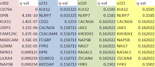
I just used the simple Cuffidiff workflow and looked at the gene_exp.diff output file for each software version. The results are quite different. Version 2.0.2 has 46 genes called "significant=yes" (multi-test adjusted q-value less than 0.05) with q-values running as low as 4.14E-10 (ok, one has a q-value of zero).  Now this is not a great result from a biostatistics standpoint, since how can you expect to get significant p-values from RNA expression levels with two samples an no replicates? But it did make for an expedient exercise, since we could take the DE genes into DAVID and look for enriched biological functions and pathways.

Then in version 2.1.1 we have two "significant=yes" genes. In version 2.2.0 we have zero significant genes, and in version 2.2.1 also zero.

The top 10 genes, ranked by q-value also differ. There are no genes in common between the top 10 list for version 2.0.2 and 2.1.1, and only the top 2 genes are shared by version 2.2.0. Thankfully, there are no differences in top genes or q-values between 2.2.0 and 2.2.1 (versions released only 2 months apart).  I'm sure that Cole Trapnell et al. are diligently improving the software, but the consequences for those of us trying to use the tools to make some sense out of biology experiments can be unsettling.


Feb 14, 2016

RNA-seq Workshop


We ran a tutorial at NYU Med Center last week on the basics of RNA-seq data analysis. This tutorial was based on the use of our High-Performance Linux cluster, so we actually presented the class as 2 sessions: A 2-hour session on basic Linux commands (for the complete novice) plus writing and submitting Sun Grid Engine scripts.  Then in the 2nd 2-hour session we focus on TopHat/Cufflinks data processing with some sample data files. So this tutorial has some parts that are rather specific to the NYUMC computing system, but it may be quit similar to what computing resources might be available at other schools and research centers.

The YouTube links to the Linux session (screencast):
https://youtu.be/M3RVfv6lUtc

and the RNA-seq session (screencast):
https://youtu.be/hksQlJLwKqohttps://youtu.be/hksQlJLwKqo

A wiki website with the Powerpoint slides and a collection of other resources:
https://genome.med.nyu.edu/hpcf/wiki/RNA-seq_tutorial_2016

Jan 28, 2016

The Tardigrade Miscalculation

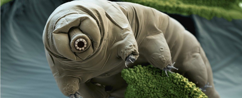
There was a lot of publicity back in November about the genome sequence of theTardigrade (Hypsibius dujardini), a small animal (0.05 – 1mm) that is somewhat similar to nematodes. These are fascinating little creatures that have been described as incredibly resistant to all manner of physical stress – high and low temperatures (reportedly from -272oC to +151oC), high pressure, complete vacuum (Tardigrades in Space = TARDIS {I kid you not}), ionizing radiation, and can survive without food or water for more than 10 years as kind of a dehydrated little lump. 

 
The reason the genome of the Tardigrade was such big news in November is that the group doing the bioinformatics analysis claimed that the genome contained 6,663 genes from bacteria, a full sixth of the genome, and twice as many horizontally transferred genes as have ever been seen in any other organism (Boothby et al, PNAS 112(52):15976-81. doi: 10.1073/pnas.1510461112. PMID: 26598659). This "weird science" observation was covered by National Geographic, Science News,  Phys.org, Meta Science News, and of course the Univ. of North Carolina press site.
 
However, it seems quite clear now that this claim about horizontal DNA from bacteria (and maybe other phyla) in the genome of the Tardigrade was wrong. In fact, another group (, , , , , , , , ,  also working on the sequence of the exact same species has rapidly published a preprint manuscript on the bioRxiv preprint server "The genome of the tardigrade Hypsibius dujardini"  that clearly refutes the claims of Boothby et al. and points out their mistakes in genome analysis: "Cross-comparison of the assemblies, using raw read and RNA-Seq data, confirmed that the overwhelming majority of the putative HGT candidates in the previous genome were predicted from scaffolds at very low coverage and were not transcribed."
 
It is quite easy to get contaminants when you are doing whole genome sequencing for a multicellular organism. You grind up your target species, extract DNA and put it into the sequencing machine. Any bacteria and other small organisms on the surface or in the gut come along for the ride and can contribute their DNA to the sequencing library. Surprisingly, a small amount of bacterial contaminating DNA (perhaps just 1%) can lead to a large number of bacterial contigs in the final genome assembly. I can think of a couple of reasons for this, based on the small size of bacterial genomes (~1 MB), vs metazoan genomes (most >100 MB). First, relative genome coverage of a contaminant bacteria will be much higher for each KB of sequence data, so the 1% of contaminating DNA may have deep coverage of a bacterial genome. Second, any two bacterial DNA fragments randomly selected from a library have a much higher chance to overlap (less complex genome), so they will assemble better.
 
There are a few QC steps that one can take on the raw data. There is a nice tool called Kraken  (Wood DE, Salzberg SL Genome Biology 2014, 15:R46) that can quickly  run through an entire FASTQ file (4 million reads per minute on a single core) and mark each read according to a set of reference genomes based on exact matching of 31 base k-mers. The Kraken team also make available a pre-built 4 GB database constructed from complete bacterial, archaeal, and viral genomes in RefSeq.  DeconSeq is another good tool to find contaminants with an easy web interface. Of course, some legitimate reads from any target organism will share k-mer sized chunks with some bacteria, viruses, etc. (and some sequences from contaminating bacteria will not be in any database), so one has to make some tough choices about what to remove from the data before assembly.
 
After assembly, there are some additional steps one can take to flag contaminants. It is extremely helpful (I would now say required) to have some RNA-seq data from the same organism. RNA-seq data is prepared using a poly-A protocol, so no bacterial RNA contaminants should be present. Any contigs (with predicted genes) that do not contain a reasonable amount of aligned RNA-seq reads are highly suspect. Any contig that has predicted genes only from a different species is clearly a red flag.
 
While the authors of the original have not (yet) published a retraction, the citation in PubMed does carry a link to the refuting article  provided by author Sujai Kumar
 
Rather than rant on about proper workflows for genome annotation (a best practices document does exist: Mark Yandell & Daniel Ence, Nature Reviews Genetics 13, 329-342 doi:10.1038/nrg3174) let me just say to the authors, the reviewers and the editors at PNAS that "EXTRODINARY CLAIMS REQUIRE EXTRODINARY EVIDENCE" (Carl Sagan). Or as said by Laplace: “The weight of evidence for an extraordinary claim must be proportioned to its strangeness.”


Jan 20, 2016

Cancer Moonshot in the Cloud

I've been reading a bit about the "Cancer Moonshot" discussion at the Davos economics conference.

http://www.weforum.org/events/world-economic-forum-annual-meeting-2016/sessions/cancer-moonshot-a-call-to-action

Naturally I'm interested in the possible increase in funding for genomics and bioinformatics research, but also the discussion of 'big data'  and sharing of genomics data are issues that I bump into all the time. It is almost impossible to overstate the amount of hoops an ordinary scientist has to jump through to obtain access or to share human genomic data that has already been published. There is an entire system of "authorized access" that requires not only that scientists swear to handle genomic data securely and make no attempt to connect genomic data back to patient identities, but also that the University (or research institute) where they work must monitor and enforce these rules. I have had to deal with this system to upload human microbiome data (DNA sequences from bacteria found in or on the human body) that are contaminated with some human DNA. [But not with the coffee beetle genome!] Then I had to apply again for authorization to view my own data to make sure it had been loaded properly.

Why is cancer genomic data protected? Unfortunately, some annoyingly clever people such as Yaniv Erlich have shown that it is possible (fairly easy in his hands) to identify people by name and address just from some of their genome sequence. Patients who agree to participate in research are supposed to be guaranteed privacy - they wanted to share information with scientists about the genetic nature of their tumors, not to share their health care records with nosy neighbors, privacy hackers and identity thieves.

Why do we need thousands of cancer genomes? One key goal of cancer research is personalized medicine - matching up people with customized treatments based on the genetics of their cancer. Current technology is pretty good for DNA sequencing of tumors - for a single cancer patient we can come up with a list of somatic mutations (found only in the tumor) for a few thousand dollars worth of sequencing effort (and a poorly measured amount of bioinformatician and oncologist time). One of the biggest challenges right now is sorting through the list of mutations to figure out which ones are important drivers of cancer growth and disease severity - and should therefore be targeted by drugs or other therapy. Some mutations are well known to be bad actors, others are new mutations in genes that have been found to be mutated in other cancers, others are complete unknowns. Data is needed from (hundreds of) thousands of tumors together with records of treatment response and other medical outcomes in order to build strong predictive models that will reliably advise the doctor about the medical importance of each observed mutation. Another challenge is the heterogeneity of cells within a single person's cancer. As DNA sequencing technology improves, investigators have started to sequence small bits of tumors, or even single cells. They observe different mutations in different cells or sub-clones. Now a key question is if the common resistance to drug treatment is a result of new mutations that occur during (or after) treament, or if the resistant cells already exist in the tumor, but are selected for growth by drug treatment. Overall, this means that precision cancer treatment may require a large number of different genome sequences from each patient, both during diagnosis and to monitor the course of treatment and post-treatment.

So cancer genomic research requires thousands of genomes (deeply sequenced for accuracy and control of artifacts), which means that each authorized investigator must download terabytes of data, and then come up with the data storage and compute power to run his or her clever analysis. In addition to the strictly administrative hurdles of applying for and maintaining an authorized access to cancer genomic data, there are the problems of data transfer, data storage, and big computing power. So the NIH (or other funding agency) has to pay once to generate the cancer genomic data, then again to store it and provide a high bandwidth web or FTP data sharing system, then again to administer the authorized access system, then again for each interested scientist to build a local computing system powerful enough to download, store, and analyze the data (and for University administrators to triple check that they are doing it properly, and again for the NIH administrators to check up on the University administrators to insure they are doing their checking properly). This is an impressive amount of redundancy and wasted effort, even for the US Government.

There is an obvious solution to this problem: 'Use the Cloud, Luke'.  A single Cloud computing system can store all cancer genomic data in a central location, together with a sufficiently massive amount of compute power so that authorized investigators can log in and run their analysis remotely. This technology already exists; Google, Amazon, Microsoft, IBM, Verizon, and at least a dozen other companies already have data centers large enough to handle the necessary data storage and compute tasks. It would be handy to build a whizz bang compute system with all kinds of custom software designed for cancer genomics, but that would take time (and government contractors). A better, faster, simpler system would just stick the genomic data in a central location and let researchers launch virtual machines with whatever software they want (or design for themselves). Amazon EC2 has this infrastructure already in place. It could be merged with the NIH authorized access system in a week-long hackathon. Cancer research Funding agencies could award Cloud compute credits (or just let people budget for Cloud computing in the standard grant application).


Cancer Moonshot:

Use the force luke - use the cloud luke